Normline

Normline is the page where analysis of FELIX and OPO infrared data are processed such as baseline correction, wavelength and power calibration In addition, one can do post-processing such as Gaussian and Multi-Gaussian line profile fitting fitting of experimental data to derive line parameters (FWHM, \(\sigma\) and amplitude).

Before proceeding further, let us familirise with different data folder structure and processed and post-processed data types for FELIX and OPO IR data.

Folder structure

graph TD
    Parent[parent-folder]

    Parent --> DATA
    Parent --> EXPORT
    Parent --> OUT

    DATA --> felix[.*felix]
    DATA --> .pow
    DATA --> .base

    EXPORT --> .dat

    OUT --> .expfit
    OUT --> .fullfit
    OUT --> other[.png, .pdf, etc]

file types

.*felix indicates any of the following: .felix, .ofelix, .cfelix or .cofelix file

Data types

Name	Description	Data source
FELIX
.felix	FELIX IR data	Instrument (Labview)
.cfelix	corrected felix	created manually (FELionGUI)
.pow	powerfile for felix	created manually (FELionGUI)
.base	baseline for felix	created manually (FELionGUI)
OPO
.ofelix	OPO IR data	Instrument (Labview)
.cbase	baseline for OPO	created manually (FELionGUI)
.cofelix	corrected ofelix	created manually (FELionGUI)
Post-processed
.dat	processed .*felix data	created manually (FELionGUI)
.expfit	Gaussian fit parameters	created manually (FELionGUI)
.fullfit	Multi-Gaussian fit parameters	created manually (FELionGUI)

Step-by-step procedure

Create baseline

Creating baseline for felix or opo IR spectrum

The procedure of processing the data are as given below in flowchart:

graph LR
  baseline[Create baseline] --> data[FELIX or OPO plot] --> post[Post processing]

As shown in above flowchart, the first step is to create a baseline

Initial steps

The measured .*felix file is copied into a folder (called parent folder as mentioned in above flowchart) followed by baseline creation Create baseline. If the parent folder is empty the following directories DATA, EXPORT and OUT are automatically generated and the copied .felix or .ofelix files are copied into the DATA folder.

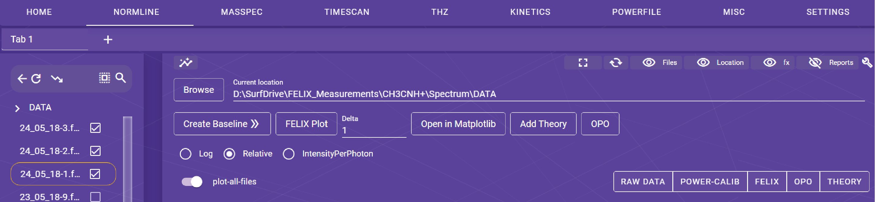
Baseline file selection

Normally files are selected by mouse left-click. However, to select a file for creating baseline one has to do ctrl + left-click. As shown in Fig 3, selected files are indicated by and the selected file for baseline correction has a solid orange coloured border.

Baseline creation

If the parent-folder is empty and this is the first time you are processing the file, then after baseline creation you should refresh () and move into DATA folder.

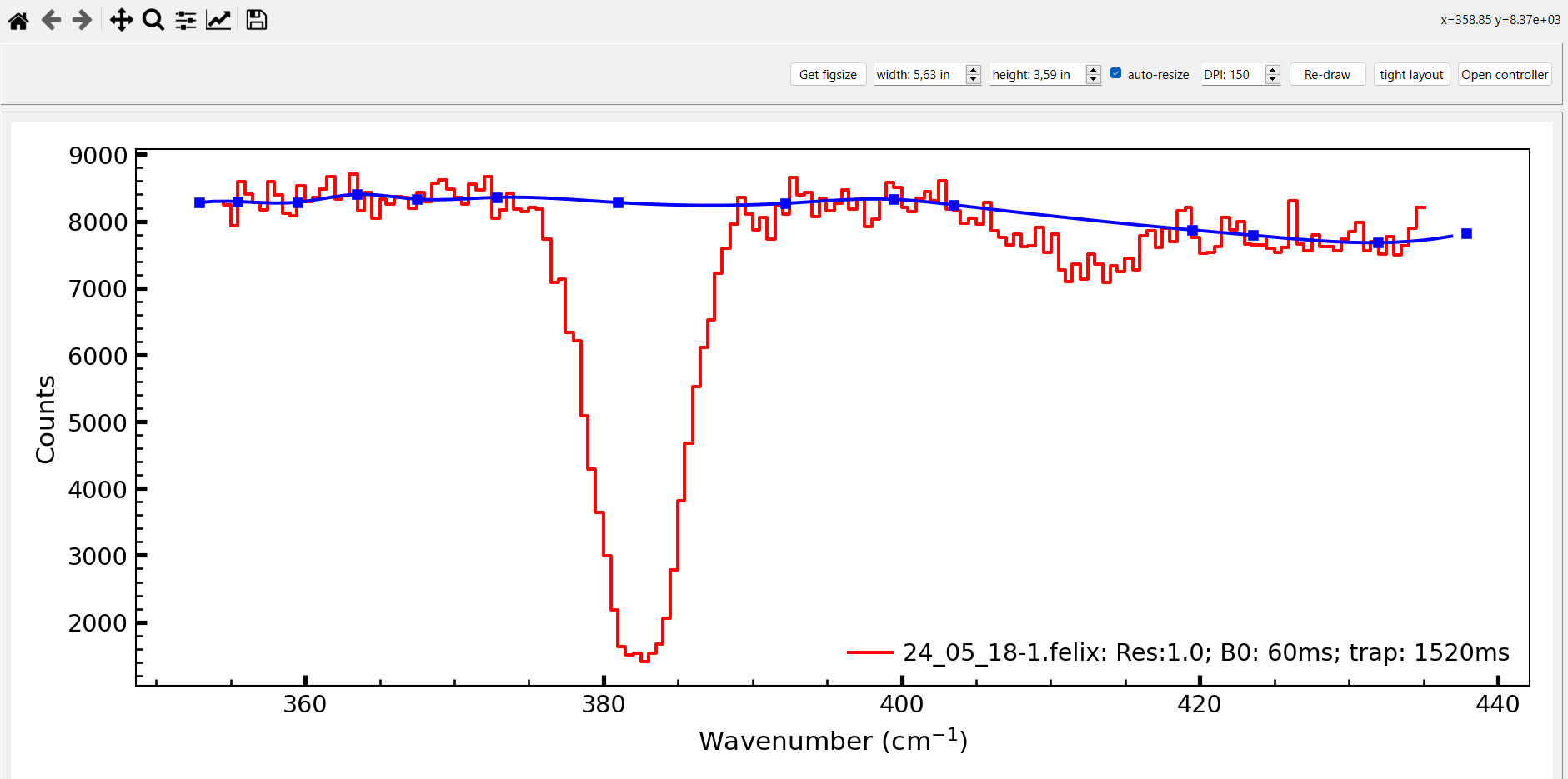
Baseline adjustment

As shown in Fig 4, the red coloured line is th measured FELIX data. While the blue coloured line corresponds to baseline which can be adjusted by dragging the solid-squared-blue-box.

The baseline is basicallya cubic spline extraploation w.r.t solid-squared-blue-box. The solid-squared-blue-box can be added or deleted, and the measured data (red coloured) can also be deleted and saved as a corrected felix file (.cfelix).

The addition and deletion can be applied when mouse is hovered over the region of interest followed by keyboard keys as shown in Table below.

keys	description
`a`	add solid-squared-blue-box point
`d`	delete solid-squared-blue-box point
`x`	delete measured-data point
`z`	undo deleted measured-data point
`r`	redo deleted measured-data point

FELIX

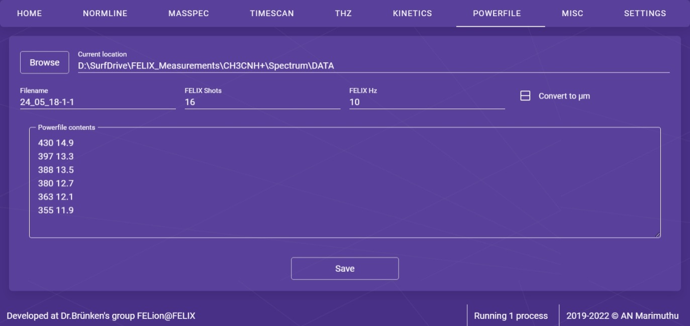
Powerfile

Create powerfile (.pow) for corresponding (.felix) file

Powerfile saving

Don't leave an empty line at the end of the powerfile. It might cause an error.

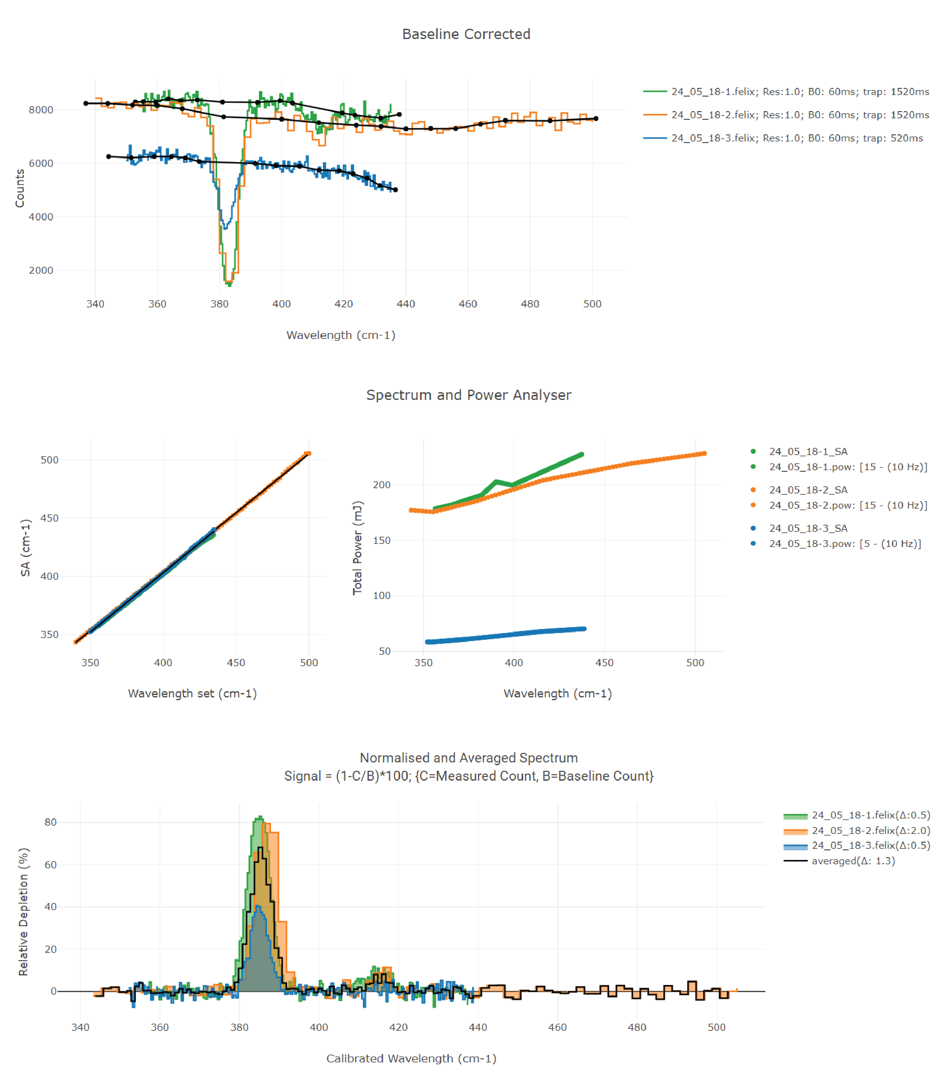
FELIX plot

graph LR
  baseline[Create baseline] --> powerfile --> felix[FELIX plot] --> post-process

As shown above, once baseline is created click on FELIX plot button to analysis FELIX IR data (from .felix file).

OPO

graph LR
  opomode[OPO MODE] --> baseline[Create baseline] --> opo[OPO plot] --> post-process

Last update: March 2, 2023